回归和分类是机器学习两个主要的类别,通常会在面试的时候,被询问这两者之间的区别。对于我,有时候我也无法说清,虽然我感觉我已经弄懂了,但是这里还是说一说自己的理解。首先,我们学过一本书《随机过程》,这里面讲到了马尔科夫链等,这是一种在时间、位置等有序列属性的数据,也就是说,这些说句不仅仅存在关系,而且存在一种序列上的前后关系,如时间、地理位置等。而分类一般核心不在于此。所以,回归问题就是一种序列预测问题,比如预测房价-时间、房间-面积、股票-时间等序列关系,通过模拟之前的序列来预测之后的序列。最简单,如线性回归,这就像我们解一元方程y=ax一样,解出a就可以了。但是,存在一个问题,这个直线是不是太直了,可能是个曲线了?或者说,更应该是是一个近似曲线的波浪线了?所以,回归的问题就开始复杂了,此时,我们开始了一些波动预测。采用的一种方式就是,对于每一个数据都有一个权重,而不是只有一个。即我们不是求单个方程,而是求解整个片段的方程,每一个点都有权值,遮掩,我们就将这个权值序列向后移动,以此来预测后来的值,即已有[1-100],那么就可以预测[2-101]来得出x=101的值,以此类推。
一、线性回归
通俗一定,线性回归就是多元以此方程组,多元指的就是多个特征值。回归最早是由达尔文的表兄弟发明的,当时他的目的是为了通过豌豆上一代的尺寸来预测下一代的尺寸,这正是回归问题。为什么叫做回归?是因为当时他发现一般人的身高虽然遗传来自父母,但是整体上还是会向均值靠近,即回归(即便他的父母很高),这个名词和这里的意义不大,但是还是有那么点意思,即任何数据都会靠近正常预测水平,不会太不靠谱(强行解释–)
- 原理
一般使用平方误差计算(因为单减误差会互相抵消):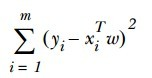
对w求导,等于0,得: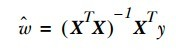
- 衡量分离的好坏,有一个方式就是通过corrcoef函数来求解相关系数,越接近0,相关性越大,说明预测越好

二、局部加权回归
线性回归有个很大的缺点,即欠拟合,太直了,不知道转弯,就是一条直线(它求得是最小均方误差的无偏估计);所以,为了防止这种情况,引入一些偏差进来,相当于做一个缓冲作用,从而降低均方误差。局部加权回归LWLR就是其中的一种
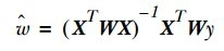
- 对每一个数据都加入一个权重系数W,最终的回归系数w就是:
- 核
这里的核类似于支持向量机中的核,通过这个核来对附近的点赋予更高的权重,一般使用的是高斯核: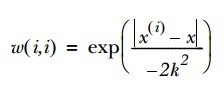
- 注意,这里的代码和线性回归不同,因为它不是一条直线,而是每个点都是一个单独计算的,所以最后的划线是片段性的。

**三、缩减系数来“理解”数据
对于分类还是回归问题,我们时常遇到数据特征比样本数量还多的情况。如果是这种情况,由于(xTx)^-1不能计算,所以是无法解决的。为了解决这个问题,我们想到了在矩阵中加入一个额外的数据,类似于补充特征。这里讲述两种方式:岭回归和lasso法(本文采用类的前向逐步回归)
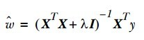
- 岭回归
- 岭回归就是在上面提到的矩阵上加一个λI 从而使矩阵非奇异(参考奇异值分解),这样就可以求逆了。之后的公式为:
- 为什么叫做缩减?因为通过引入惩罚项后,可以限制所有w的和,这样就能够减少不重要的参数,在统计学上就叫做缩减,这样能更好的理解数据(奇异值分解就是这个作用,提取出关键的信息点)
- 标准化问题:这里对特征进行了标准化处理,以使特征具有相同的重要性(这里的处理类似于归一化,但是在归一化的基础上又除以了跨度值);而对于结果y只有归一化。

- lasso
- 这种方式通过对每一个点进行上下浮动取值,来定点优化;从而遍历优化所有的w

- 四、代码*
- regression.py
1 | """ |
- 测试段:
1 | """ |
1 | """ |
1 | """ |
1 | """ |